Grasslands are important for global biodiversity, food security, and climate change analyses, which makes mapping and monitoring of vegetation changes in grasslands necessary to better understand, sustainably manage, and protect these ecosystems. However, grassland vegetation monitoring at spatial and temporal resolution relevant to land management (e.g., ca. 30-m, and at least annually over long time periods) is challenging due to complex spatio-temporal pattern of changes and often limited data availability. Here we assess both shortand long-term changes in grassland vegetation cover from 1987 to 2019 across the Caucasus ecoregion at 30-m resolution based on Cumulative Endmember Fractions (i.e., annual sums of monthly ground cover fractions) derived from the full Landsat record, and temporal segmentation with LandTrendr. Our approach combines the benefits of physically-based analyses, missing data prediction, annual aggregations, and adaptive identification of changes in the time-series. We analyzed changes in vegetation fraction cover to infer the location, timing, and magnitude of vegetation change episodes of any length, quantified shifts among all ground cover fractions (i.e., green vegetation, non-photosynthetic vegetation, soil, and shade), and identified change pathways (i.e., green vegetation loss, desiccation, dry vegetation loss, revegetation green fraction, greening, or revegetation dry fraction). We found widespread long-term positive changes in grassland vegetation (32.7% of grasslands), especially in the early 2000s, but negative changes pathways were most common before the year 2000. We found little association between changes in green vegetation and meteorological conditions, and varied relationships with livestock populations. However, we also found strong spatial heterogeneity in vegetation dynamics among neighboring fields and pastures, demonstrating capability of our approach for grassland management at local levels. Our results provide a detailed assessment of grassland vegetation change in the Caucasus Ecoregion, and present an approach to map changes in grasslands even where availability of Landsat data is limited.
File: 1-s2.0-S2666017221000225-main.pdf
Global change analyses are facilitated by the growing number of remote-sensing datasets that have both broad spatial extent and repeated observations over decades. These datasets provide unprecedented power to detect patterns of time trends involving information from all pixels on a map. However, rigorously testing for time trends requires a solid statistical foundation to identify underlying patterns and test hypotheses. Appropriate statistical analyses are challenging because environmental data often have temporal and spatial autocorrelation, which can either obscure underlying patterns in the data or suggest false associations between patterns in the data and independent values used to explain them. Existing statistical methods that account for temporal and spatial autocorrelation are not practical for remote-sensing datasets that often contain millions of pixels. Here, we first analyze simulated data to show the need to account for both spatial and temporal autocorrelation in time-trend analyses. Second, we present a new statistical approach, PARTS (Partitioned Autoregressive Time Series), to identify underlying patterns and test hypotheses about time trends using all pixels in large remote sensing datasets. PARTS is flexible and can include, for example, the effects of multiple independent variables, such as land-cover or latitude, on time trends. Third, we use PARTS to analyze global trends in NDVI, focusing on trends in pixels that have not experienced land-cover change. We found that despite the appearance of overall increases in NDVI in all continents, there is little statistical support for these trends except for Asia and Europe, and only in some land-cover classes. Furthermore, we found no overall latitudinal trend in greening for any continent, but some latitude by land-cover class interactions, implying that latitudinal patterns differed among land-cover classes. PARTS makes it possible to identify patterns and test hypotheses that involve the aggregate information from many pixels on a map, thereby increasing the value of existing remote-sensing datasets.
File: 1-s2.0-S0034425721003989-main.pdf
Bird species richness is highly dependent on the amount of energy available in an ecosystem, with more available
energy supporting higher species richness. A good indicator for available energy is Gross Primary Productivity
(GPP), which can be estimated from satellite data.
Our question was how temporal dynamics in GPP affect bird species richness. Specifically, we evaluated the
potential of the Dynamic Habitat Indices (DHIs) derived from MODIS GPP data together with environmental and
climatic variables to explain annual patterns in bird richness across the conterminous United States. By focusing
on annual DHIs, we expand on previous applications of multi-year composite DHIs, and could evaluate lag-effects
between changes in GPP and species richness.
We used 8-day GPP data from 2003 to 2013 to calculate annual DHIs, which capture three aspects of vegetation
productivity: (1) annual cumulative productivity, (2) annual minimum productivity, and (3) annual
seasonality expressed as the coefficient of variation in productivity. For each year from 2003 to 2013, we
calculated total bird species richness and richness within six functional guilds, based on North American
Breeding Bird Survey data.
The DHIs alone explained up to 53% of the variation in annual bird richness within the different guilds
(adjusted deviance-squared D2adj = 0.20–0.52), and up to 75% of the variation (D2adj = 0.28–0.75) when
combined with other environmental and climatic variables. Annual DHIs had the highest explanatory power for
habitat-based guilds, such as grassland (D2adj = 0.67) and woodland breeding species (D2adj = 0.75). We found
some inter-annual variability in the explanatory power of annual DHIs, with a difference of 5–7 percentage
points in explained variation among years in DHI-only models, and 3–7 points for models combining DHI,
environmental and climatic variables. Our results using lagged year models did not deviate substantially from
same-year annual models.
We demonstrate the relevance of annual DHIs for biodiversity science, as effective predictors of temporal
variation in species richness patterns. We suggest that the use of annual DHIs can improve conservation planning,
by conveying the range of patterns of biodiversity response to global changes, over time.
File: Hobi-et-al-2021_BirdSpeciesRichness_DynamicHabIndices_EcolIndicators.pdf
Maps are a key instrument and important data source for a wide range of research from global modeling to detailed ecological studies of a specific species. However different scales of tasks require proper instruments including a suitable maps detalization. For instance, a scientist who is interested in the general trends of agriculture abandonment may not have to pay too much attention to which specific fields are not in use anymore. However, for a conservation biologist studying a rare species, detailed maps of habitats, such as abandoned crops, is critical. However, it is difficult to make such detailed maps for large areas. Global maps are many, but they lack necessary details, while fine-scale maps only cover small areas if they exist at all. Unfortunately, using inappropriate scale of the input information either makes the results too general to be sensible or leads to incorrect conclusions.
In practical terms, precise mapping is a matter of balance of time and efforts versus the desired quality of results. The more accurate is a map the more resources are required to make it. But the amount of the resources necessary for creating a good map for a large area may be beyond what project managers can afford.
Coming back to the abandonment and land cover mapping, the maps are important for a variety of tasks including economic (re)development, nature conservation, and agriculture improvements. Thus, the absence of proper maps could make ecological and economic problems even worse.
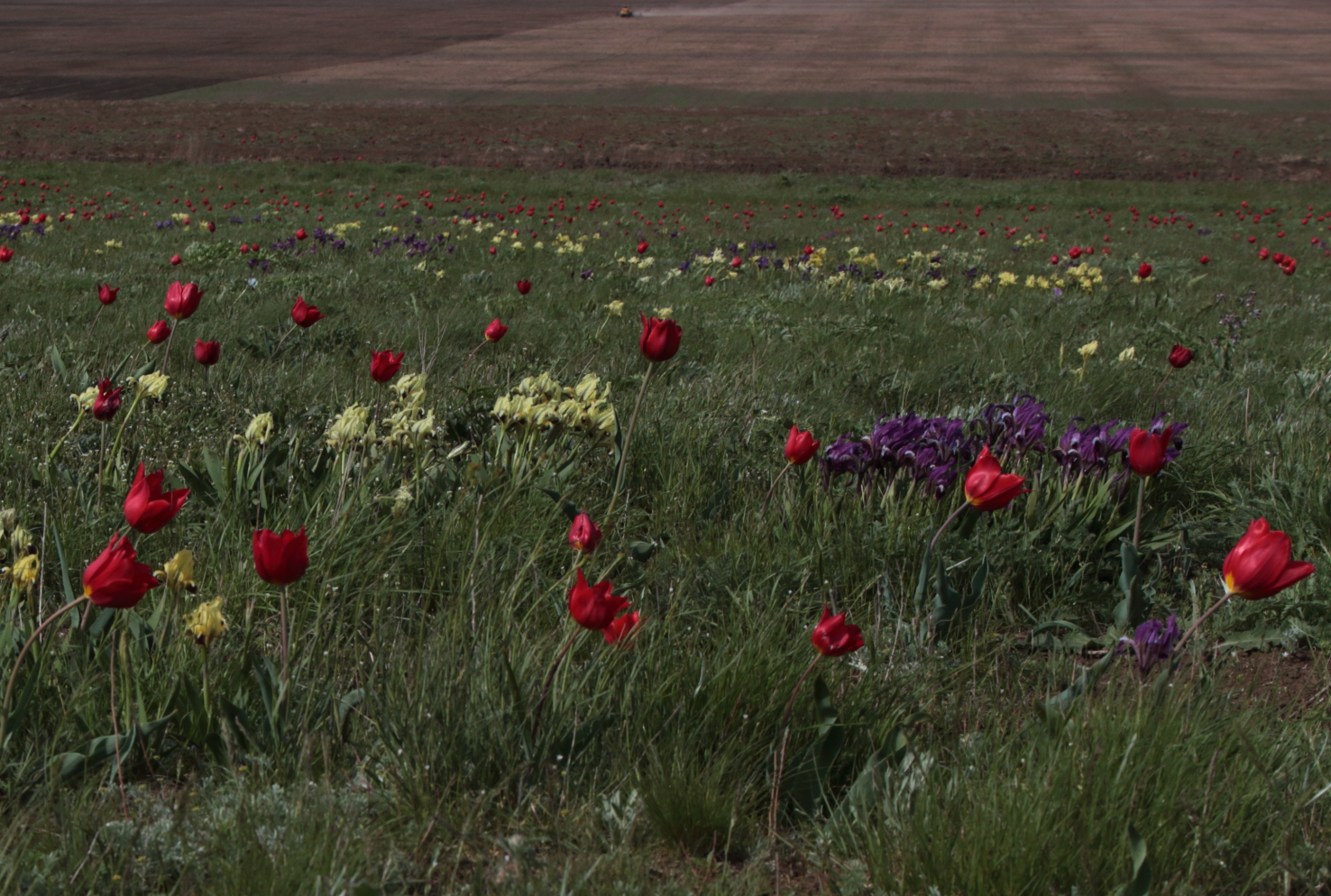
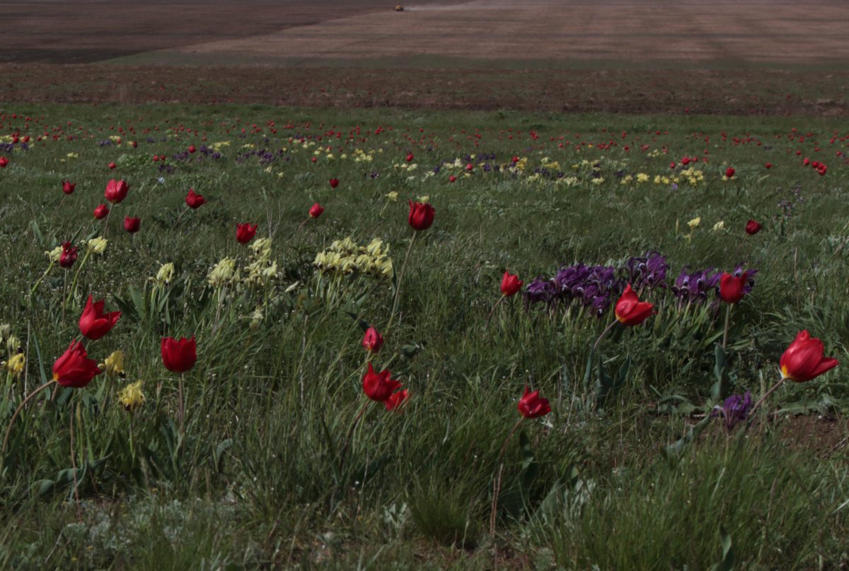
Part of my research is about the level of accuracy we could (or should) achieve when mapping large areas. I have chosen the Eurasian Steppe as a test site because it is vast, large areas of abandonment, as well as permanently used field,) and rich diversity of natural vegetation. At the same time, it is one of the most transformed landscapes in Eurasia where biodiversity conservation and preserving intact steppes as the source of both rare and dominant native species to re-habit the man-made vacuum is a top priority. What makes the mapping of these areas challenging though is that the natural vegetation, mainly grasses and herbs, is spectrally very similarly to agriculture in satellite images.
I am planning to test several mapping techniques taking into account the advantages of each and adjust them to specific conditions of the steppe. The random forest algorithm is easy and fast enough to make initial maps. These maps show general land cover of an area and allow to reveal sources of mismapping. The segmentation algorithm is helpful in drawing more clear borders but fails to distinguish objects that have similar reflection while belonging to different classes. The understanding of general structure gained from the initial maps gives better reasons to divide a large heterogeneous area into smaller and more solid parts where differences between the mapping classes are higher than in-class variability. Ultimately, I hope to achieve two results. The first is understanding of how to combine existing methods to improve the whole map quality. The second is to create maps suitable for ecological research, preserving biodiversity and the establishment of new protected areas.

Over the course of a year, vegetation and temperature have strong phenological and seasonal patterns, respectively, and many species have adapted to these patterns. High inter-annual variability in the phenology of vegetation and in the seasonality of temperature pose a threat for biodiversity. However, areas with high spatial variability likely have higher ecological resilience where inter-annual variability is high, because spatial variability indicates presence of a range of resources, microclimatic refugia, and habitat conditions. The integration of inter-annual and spatial variability is thus important for biodiversity conservation. Areas where spatial variability is low and inter-annual variability is high are likely to limit resilience to disturbance. In contrast, areas of high spatial variability may be high priority candidates for protection. Our goal was to develop spatiotemporal remotely sensed indices to identify hotspots of biodiversity conservation concern. We generated indices that capture the inter-annual and spatial variability of vegetation greenness and land surface temperature and integrated them to identify areas of high, medium, and low biodiversity conservation concern. We applied our method in Argentina (2.8 million km2), a country with a wide range of climates and biomes. To generate the inter-annual variability indices, we analyzed MODIS Enhanced Vegetation Index (EVI) and Land Surface Temperature (LST) time series from 2001 to 2018, fitted curves to obtain annual phenological and seasonal metrics, and calculated their inter-annual variability. To generate the spatial variability indices, we calculated standard deviation image texture of Landsat 8 EVI and LST. When we integrated our inter-annual and spatial variability indices, areas in the northeast and parts of southern Argentina were the hotspots of highest conservation concern. High inter-annual variability poses a threat in these areas, because spatial variability is low. These are areas where management efforts could be valuable. In contrast, areas in the northwest and central-west are where protection should be strongly considered because the high spatial variability may confer resilience to disturbance, due to the variety of conditions and resources within close proximity. We developed remotely sensed indices to identify hotspots of high and low conservation concern at scales relevant to biodiversity conservation, = which can be used to target management actions in order to minimize biodiversity loss.
File: RSE_Silveira_2021.pdf
Environmental heterogeneity enhances species richness by creating niches and providing refugia. Spatial variation in climate has a particularly strong positive correlation with richness, but is often indirectly inferred from proxy variables, such as elevation and related topographic heterogeneity indices, or derived from interpolated coarsegrain weather station data. Our aim was to develop new remotely sensed metrics of relative temperature and thermal heterogeneity, compare them with proxy measures, and evaluate their performance in predicting species richness patterns. We analyzed Landsat 8’s Thermal Infrared Sensor data, calculated two thermal metrics during summer and winter, and compared their seasonal spatial patterns with those of elevation and topographic heterogeneity. We fit generalized least squares models to evaluate each variable’s effect in predicting seasonal bird richness using data from the North American Breeding Bird Survey. Generally speaking, neither elevation nor topographic heterogeneity were good proxies for temperature or thermal heterogeneity, respectively. Relative temperature had a non-linear relationship with elevation that was negatively quadratic in summer, but slightly positively quadratic in winter. Topographic heterogeneity had a stronger positive relationship with thermal heterogeneity in winter than in summer. The magnitude and direction of elevation–temperature and topographic heterogeneity–thermal heterogeneity relationships in each season also varied substantially across ecoregions. Remotely sensed metrics of relative temperature and thermal heterogeneity improved the predictive performance of species richness models, and both thermal variables had significant effects on bird richness that were independent of elevation and topographic heterogeneity. Thermal heterogeneity was positively related to total breeding bird richness, migrant breeding bird richness and resident bird richness, whereas topographic heterogeneity was negatively related to total breeding richness and unrelated to migrant or resident bird richness. Because thermal and topographic heterogeneity had contrasting seasonal patterns and effects on richness, they must be carefully contextualized when guiding conservation priorities.
File: ecog.05520.pdf
After 1991, major events, such as the collapse of socialism and the transition to market economies, caused land use change across the former USSR and affected forests in particular. However, major land use changes may have occurred already during Soviet rule, but those are largely unknown and difficult to map for large areas because 30-m Landsat data is not available prior to the 1980s. Our goal was to analyze the rates and determinants of forest cover change from 1967 to 2015 along the Latvian-Russian border, and to develop an object-based image analysis approach to compare forest cover based on declassified Corona spy satellite images from 1967 with that derived from Landsat 5 TM and Landsat 8 OLI images from 1989/1990 and 2014/2015. We applied Structurefrom- Motion photogrammetry to orthorectify and mosaic the scanned Corona images, and extracted forest cover from Corona and Landsat mosaics using object-based image analysis in eCognition and expert classification. In a sensitivity analysis, we tested how the scale parameters for the segmentation affected the accuracy of the change maps. We analyzed forest cover and forest patterns for our full study area of 22,209 km2, and applied propensity score matching approach to identify three Latvian-Russian pairs of 15 × 15 km cells, which we compared. We attained overall classification accuracies of 92% (Latvia) and 93% (Russia) for the forest/non-forest change maps of 1967–1989, and 91% (Latvia) and 93% (Russia) for 1989–2015, and our results were robust in regards to the segmentation scale parameter. Sample-based forest cover gain from 1967 to 1989 differed notably between the two countries (18.5% in Latvia and 23.6% in Russia), but was generally much higher prior to 1989 than from 1989 to 2015 (8.7% in Latvia and 9.7% in Russia). Furthermore, we found rapid de-fragmentation of forest cover, where forest core area increased, and proportions of isolated patches and forest corridors decreased, and this was particularly pronounced in Russia. Our findings highlight the need to study Soviet-time land cover and land use change, because rural population declines and major policy decisions such as the collectivization of agricultural production, merging of farmlands and agricultural mechanization led already during Soviet rule to widespread abandonment and afforestation of remote farmlands. After 1991, government subsidies for farming declined rapidly in both countries, but in Latvia, new financial aid from the EU became available after 2001. In contrast, remoteness, lower population density, and less of a legacy of intensive cultivation resulted in higher rates of forest gain in Russia. Including Corona imagery in our object-based image analysis workflow allowed us to examine half a century of forest cover changes, and that resulted in surprising findings, most notably that forest area gains on abandoned farm fields were already widespread during the Soviet era and not just a postsocialist land use change trend as had been previously reported.
File: 1-s2.0-S0034425720303801-main.pdf
European Russia rapidly transitioned after the collapse of the Soviet Union from state socialism to a market economy. How did this political and economic transformation interact with ecological conditions to determine forest loss and gain? We explore this question with a study of European Russia in the two decades following the collapse of the Soviet Union. We identify three sets of potential determinants of forest-cover change—supply-side (environmental), demand-side (economic), and political/administrative factors. Using new satellite data for three distinct types of forest-cover change—logging, forest fires, and forest gain—we quantify the relative importance of these variables in province-level regression models during periods of a) state collapse (1990s), and b) state growth (2000s). The three sets of covariates jointly explain considerable variation in the outcomes we examine, with size of forest bureaucracy, autonomous status of the region, and prevalence of evergreen forests emerging as robust predictors of forest-cover change. Overall, economic and administrative variables are significantly associated with rates of logging and reforestation, while environmental variables have high explanatory power for patterns of forest fire loss.
File: 1-s2.0-S0264837719312153-main.pdf
Cropland abandonment is a widespread land-use change, but it is difficult to monitor with remote sensing because it is often spatially dispersed, easily confused with spectrally similar land-use classes such as grasslands and fallow fields, and because post-agricultural succession can take different forms in different biomes. Due to these difficulties, prior assessments of cropland abandonment have largely been limited in resolution, extent, or both. However, cropland abandonment has wide-reaching consequences for the environment, food production, and rural livelihoods, which is why new approaches to monitor long-term cropland abandonment in different biomes accurately are needed. Our goals were to 1) develop a new approach to map the extent and the timing of abandoned cropland using the entire Landsat time series, and 2) test this approach in 14 study regions across the globe that capture a wide range of environmental conditions as well as the three major causes of abandonment, i.e., social, economic, and environmental factors. Our approach was based on annual maps of active cropland and non-cropland areas using Landsat summary metrics for each year from 1987 to 2017. We streamlined perpixel classifications by generating multi-year training data that can be used for annual classification. Based on the annual classifications, we analyzed land-use trajectories of each pixel in order to distinguish abandoned cropland, stable cropland, non-cropland, and fallow fields. In most study regions, our new approach separated abandoned cropland accurately from stable cropland and other classes. The classification accuracy for abandonment was highest in regions with industrialized agriculture (area-adjusted F1 score for Mato Grosso in Brazil: 0.8; Volgograd in Russia: 0.6), and drylands (e.g., Shaanxi in China, Nebraska in the U.S.: 0.5) where fields were large or spectrally distinct from non-cropland. Abandonment of subsistence agriculture with small field sizes (e.g., Nepal: 0.1) or highly variable climate (e.g., Sardinia in Italy: 0.2) was not accurately mapped. Cropland abandonment occurred in all study regions but was especially prominent in developing countries and formerly socialist states. In summary, we present here an approach for monitoring cropland abandonment with Landsat imagery, which can be applied across diverse biomes and may thereby improve the understanding of the drivers and consequences of this important land-use change process.
File: 1-s2.0-S0034425720302431-main.pdf
The United States (U.S.) federal government provides imagery obtained by federally funded Earth Observation satellites typically at no cost. For many years Landsat was an exception to this trend, until 2008 when the United States Geological Survey (USGS) made Landsat data accessible via the internet for free. Substantial increases in downloads of Landsat imagery ensued and led to a rapid expansion of science and operational applications, serving government, private sector, and civil society. The Landsat program hence provides an example to space agencies worldwide on the value of open access for Earth Observation data and has spurred the adaption of similar policies globally, including the European Copernicus Program. Here, we describe important aspects of the Landsat free and open data policy and highlight the importance and continued relevance of this policy.
File: 1-s2.0-S0034425719300719-main.pdf