Posted 02/8/21
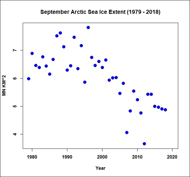
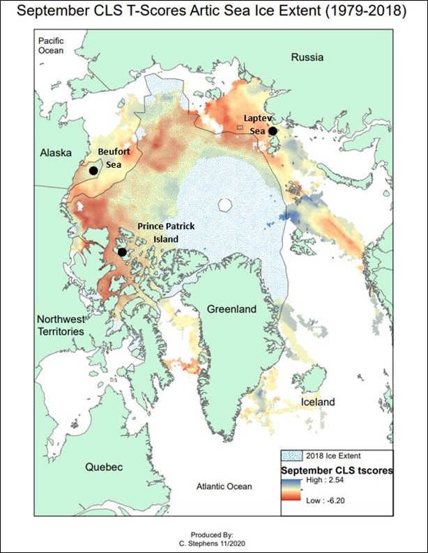
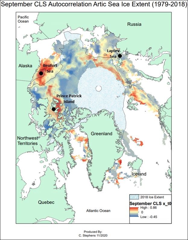
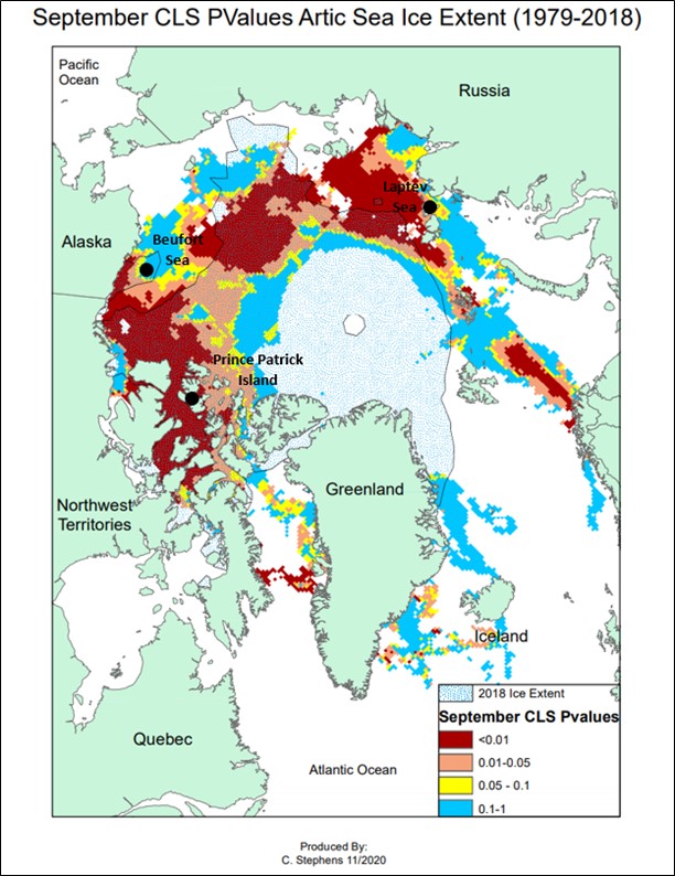
We analyzed the SMMR/SMMI archive (1979-2020) to assess trends in Arctic sea ice extent. We quantified sea ice extent as the number of days of ice coverage in 25-km pixels in September, when Arctic sea ice is at its minima. By fitting constrained least squares regression, we accounted for temporal autocorrelation in the trends. Three regions; the Beaufort Sea, the Laptev Sea, and Prince Patrick Island were found to have highly autocorrelated trends in sea ice loss.
Rapid warming of the Arctic is expected to cause substantial loss arctic sea ice volume and surface area. This will have numerous ecological and economic implications including habitat loss for sensitive species such as Polar Bear and Walrus, accelerated heating of the Arctic Ocean due to lowered albedo, and heightened shipping activity within the Arctic due to the increased availability of ice-free ports.
Sea ice loss has already been rapid, particularly during the summer months (Figure 1), and that this trend will only accelerate. The question is when and when exactly these losses occurred, and if observed trends are statistically significant. A major reason why this is difficult to ascertain is spatial and temporal autocorrelation, that is the influence nearby ice, and of previous ice abundance has on current conditions. We account for autocorrelation in our analyses of Arctic sea ice loss using a constrained least squares autoregressive model that predicts ice abundance based on the prior year’s conditions.
We found that three regions have experienced significant and highly temporally autocorrelated sea ice loss; a) the Laptev Sea near Severnaya Zemlya, Russia, b) the Beaufort Sea near northeastern Alaska, USA, and c) the Arctic Ocean near Prince Patrick island, Canada (Maps 1, 2, 3). Our next step is to apply a Generalized Least Squares model intended to detect spatial patterns in trends of sea ice loss.
Story by Stephens, Connor